The Problem

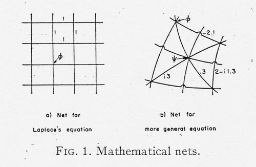
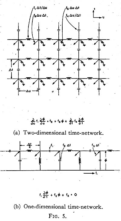
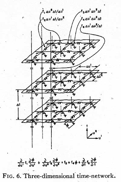
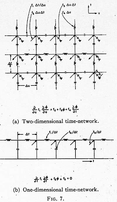
The equivalent circuits consist of a configuration of coils repeated along one, two, or three axes. The final shape of the network is the same as the shape of the field to be analyzed. While the illustrations will refer to two-dimensional networks, all rules and formulae are equally valid for one- and three-dimensional networks.

In analyzing a field, at first it should be divided into a very few subdivisions only. After its field distribution has been calculated, it should be subdivided into a finer mesh then, if needed, into still finer meshes. In most problems it will be necessary to introduce fine meshes only in certain portions, usually around corners.

The problem in all cases is the following:

(1) Given the boundary conditions in the form of known currents flowing in some of the coils and in the form of known absolute potentials at certain junctions.

(2) Find the absolute potentials of all junctions and the currents flowing in all conductors.

In linear problems the impedances of all coils are also known. In non-linear problems only some of the impedances are known, while the value of others are functions of the as yet unknown absolute, potentials and their derivatives. Some of the junction currents also may be functions of the potentials.


A Preliminary Step

In most networks the absolute potentials of the junctions have a physical meaning. In particular: (1) In the electromagnetic field it is E_y, the field- intensity, along the y-direction, or H_y.
(2) In elasticity it is the total displacement u or v.

(3) In hydrodynamics it may be the stream- function ψ or velocity potential φ etc.

In all methods of attack as a preliminary step a tentative potential distribution at the junctions is assumed. Usually an intelligent guess may be made and if the guess is far off, that only entails more labor, without, however, influencing the correctness of the final answer. (Instead of the potential distribution, a guess may be made at the current-distribution.) Of course in linear problems this preliminary step may be done on a Network Analyzer, even though only a very few units are available, or the results of an approximate or exact solution may be used as starting points.

Once the absolute potentials at all the junctions are assumed to be known, it is always possible to calculate the currents flowing in all the coils. In non-linear problems at first the coil admittances and junction currents must be calculated from the known potentials, then the coil currents. Examples of non-linear networks are those of the potential flow of a compressible fluid in the physical plane, given in reference 7, Figs. 10 and 11.

The method of attack is based upon the fact that if the correct potential distribution is assumed and if all currents in the coils have been calculated then:
(1) The sum of the currents

entering each junction is zero.
(2) The weighted average of the potentials of neighboring junctions is equal to the potential of the central junction.

Three types of numerical calculations may be performed depending upon whether the weighted average of the currents entering a junction, or of the voltages surrounding a junction, or of both, are calculated.

Because of the bad guess, however, actually at no time will the above conditions be fulfilled at all junctions simultaneously. The purpose of the calculation is to reduce the difference in the entering and departing currents (or the difference between the surrounding and the central potentials) as close to zero as possible at all junctions.

This difference in the currents will be called the "unbalanced current" i_u , and the difference in the voltages the "unbalanced vOltage" e_u . It should be noted that:
(1) The "unbalanced voltages" offer a clue on how much to change the guessed-at voltages to reduce the error.
(2) The "unbalanced currents" give an indication of how much the guessed-at values differ from the correct values.


Calculation of the "Unbalanced" Currents and Voltages



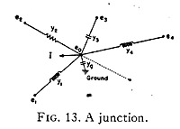
The unbalanced currents i_u at each junction are best calculated by summing up the currents entering it. To find the unbalanced voltage. e_u at a junction whose absolute potential is e₀, let Fig. 13 be considered. The unbalanced current may also be found by

If it is assumed that no unbalanced currents exist (i_u = 0) then the correct value of the assumed potential e₀would be E, the weighted average

Since e₀ is assumed instead of E, the unbalanced voltage is

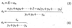
Hence the relation between and e_u at every junction is

is the sum of the admittances of all the coils leading to the junction.


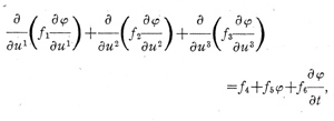
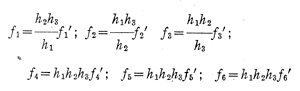
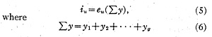
The Field Equations of Maxwell

In Laplace's equation, where y₁ = y₂ = y₃ = y₄ = 1 and y_g = I = 0,


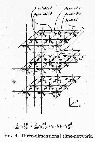
In Maxwell's equation, in rectangular coordinates, Fig. 4, where y₁ = y₂ = y₃ = y₄ = y_L and y_g = y_c (acapacitance, a negative number),



a number less than four.

That is, finding the unbalanced currents and voltages for the field equations of Maxwell in rectangular coordinates is no more complicated than finding the same quantities in Laplace's equation (i.e., the number 4 is replaced by k). It will be found in most problems that the general equations (1), (4), and (2) for finding i_u,e_u and E may be considerably simplified.


The Method of Unbalanced Currents and Voltages

One of the quickest ways (if not the quickest) to solve a complicated network is the following:

1. Assume (or measure by a Network Analyzer) the potentials at all junctions.
2. Calculate at all junctions the unbalanced currents i_u and the unbalanced voltages e_u.
3. Knowing the whole set of unbalanced quantities at the junctions assume a new set of potentials that are more correct. In general, where e _u is positive, the potential should decrease and with negative e _u it should increase.
4. Calculate over again the whole set of new unbalanced quantities at every junction.

Such successive guesses and calculations should reduce the unbalanced quantities below any desired amount. Plotting curves of the unbalanced currents, voltages, and of the guessed-at values at frequent intervals helps to speed up the convergence.


Examples of Unbalanced Quantity Calculations

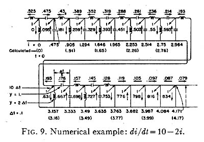
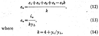
Let a square wave guide or cavity resonator, by a conducting surface that extends to infinity in the y direction, be divided into sixteen squares. The net of coils in each square consists of two inductances (z=0.8 or y=1.25) and a ground capacitor (z=1.3 or y=0.77). The currents in the inductance represent E_x and E_z, while the voltages across the capacitors represent H_y.



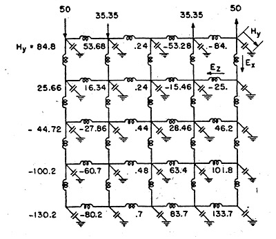
Fig. 14, bounded in the x-z plane on three sides.

For boundary conditions, it is assumed that at the open end (upper end) a sinusoidal current distribution in space, E_x, is impressed. As a result, a sinusoidal potential distribution H_y appears at the junctions. Neither the magnitude nor the wave-length of H_y is known.

Tentatively let the values shown on Fig. 14 be assumed as the junction potentials H _y. (Actually these values were found on the Network Analyzer.)



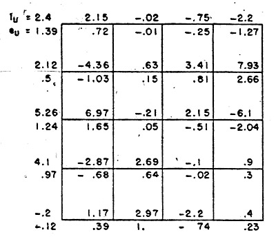
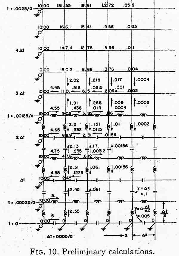
FIG. 15. Unbalanced currents and voltages on the wave guide network.

Figure 15 gives the unbalanced currents and voltages that will have to be liquidated. It should be noted that the greatest unbalanced junction current is 7.93 amperes. As the greatest coil current is 102.8 amperes, that represents an 8 percent inaccuracy.

Knowing the unbalanced currents and voltages at every junction, a new set of junction potentials may now be assumed.



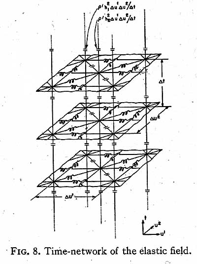
For an elastic stress problem of a beam, a set of junction potentials (representing displacements in the x or y directions) and a set of unbalanced currents are shown in Fig. 16 (reproduced from Carter (8)).


The Method of Weighted Averages

Instead of attempting to reduce the unbalanced quantities simultaneously at all junctions, it is possible to reduce them at one junction at a time. Two such methods will be shown .

(1)The unbalanced current and voltage are reduced to zero at a junction without compensating at the neighboring junctions (the method of weighted averages).
(2) Each time the unbalancect current or voltage is reduced at a junction, the unbalanced quantities at the neighboring junctions are compensated simultaneously (the relaxation method).

The first method is especially valuable when the guessed at value of potentials differs from the correct value only at isolated points or regions. Such is the case usually in Network Analyzer solutions when at some junctions the instrument reading is incorrect or the board unit happened to be incorrectly set. The steps are as follows:

(1) Assume (or measure) the potentials at all junctions.
(2) Calculate E, the weighted average, at any junction by Eq. (2).
(3) Replace e₀ by E.

In the previous method e₀ was not replaced by E. Only the corresponding e_u for each e₀ was calculated, leaving e₀ undisturbed.

It is customary to start at one corner of the network and change in succession all e₀ to E, utilizing the already corrected potentials wherever they are available. A disadvantage of this method is that it is equivalent to reducing the unbalanced potential e_u at each junction immediately to zero.

A more advantageous procedure is to replace at each junction the value of e₀ not by E but by a value larger than E, or smaller (depending on the value of the neighboring potentials) leaving thereby at each junction an unliquidated e _u that is within the allowable limit of error.

In non-linear problems it is often possible to plot curves which give outright the value of E for given neighboring potentials (or rather for given potential-differences between neighboring junctions). If difficulties in the convergçnce arise, in place of E a value larger (or smaller) should be used.


The Relaxation Method

The relaxation method reduces the unbalanced currents or voltages at one junction at a time toward zero in a systematic manner. It is based upon the fact that whenever the absolute potential of a particular junction is changed, the unbalanced currents and voltages change only at that particular junction and at all the neighboring junctions to which a coil leads, while everywhere else the unbalanced junction currents remain unchanged.


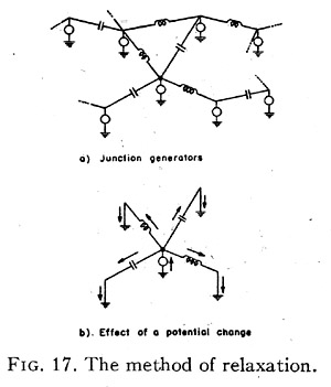
This fact may be seen by introducing a set of hypothetical generators so that (Fig. 17a):

(1) At every junction a generator with zero impedance is assumed to be connected to the ground.
(2) The generator voltage is equal to the absolute potential of the junction.
(3) The generator current to ground is equal the to unbalanced current existing at that junction.

By the introduction of these hypothetical generators the network remains unchanged and is now capable of performing new feats that it couldn't do otherwise. Since the generators have zero impedance to ground, whenever one of the generator voltage is changed, currents can flow from this generator only to the neighboring grounds. (Fig. 17b). No change of currents exist anywhere else in the network.

Hence, the unbalanced currents are reduced in two steps:

(1) Add (or subtract) a certain number of volts to the potential of a junction.
(2) Find the new unbalanced currents (or voltages) at that junction and in the neighboring junctions.

Whether the unbalanced currents, or voltages, or both should be calculated depends on the problem at hand.


The "Unbalanced-Current Patterns"

The work involved in this last step may be greatly reduced in linear problems by the device of the "unbalanced-current pattern". This device consists of calculating once for all the change in the unbalanced junction currents caused by a change of one volt at every junction. (With non- linear coils this device cannot be used.) Two cases may be distinguished:

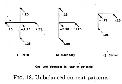
(1) If the square nets of impedances throughout the network are identical, then each junction that does not lie on the boundary, has identical current-pattern. Similarly all horizontal, also all vertical, boundary junctions have identical pattern, as well as all corners. The various patterns for the wave- guide example are given in Fig. 18 (plus current flows into a junction, minus current flows out of a junction).
(2) If the impedances vary from point to point, then for every junction a different current-pattern has to be established.

In analogy to the "unbalanced current patterns" it is possible to set up "unbalanced voltage patterns" by multiplying each i_u by its respective Σy.


The Numerical Reduction

It should be noted that every time a junction- voltage is decreased, the junction currents at the neighboring junctions increase, but at the junction itself it decreases. And the decrease is always greater than the increase (—4.23 amp. as against 1.25 amp.).

Hence the general procedure is to decrease (or increase) the unbalanced currents at those junctions where the unbalance is the greatest. Two columns should be established at every junction:
(1) One column showing the change in the absolute potential assumed.
(2) The other showing the new unbalanced currents (or voltages, or both).

There will be many more entries in the current column since the current varies also whenever the potential at a neighboring junction varies.


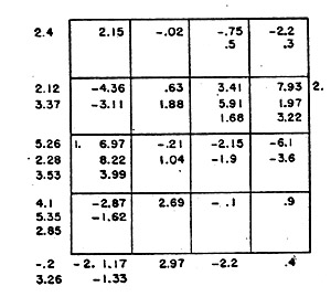
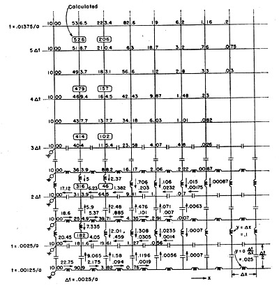
Fig. 19. Reduction of unbalanced currents to one-half of their value (from 8 percent to 4 percent).

Fig. 19 shows the steps necessary to reduce in the example of Fig. 15 the unbalanced currents from 8 percent to 4 percent. By changing the voltages only at five junctions, the accuracy of the a.c. Network Analyzer results has been increased 100 percent.



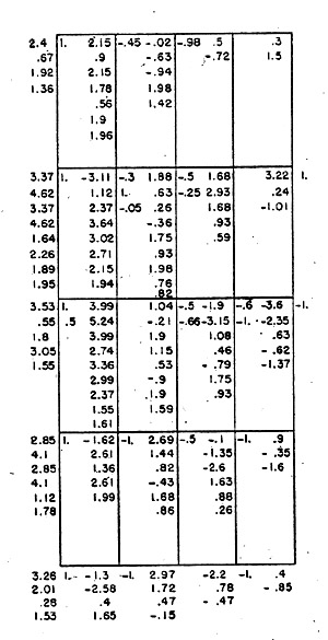
Fig. 20. Reduction of unbalanced currents to one-fourth of their value (from 4 percent to 2 percent).

Figure 20 shows the steps necessary to reduce the unbalanved currents from 4 percent to 2 percent. Now 24 changes had to be assumed instead of five to increase the accuracy by another 100 percent. To reduce the unbalanced currents from 2 percent to 1 percent probably the same or greater number of changes would be necessary.

It is emphasized that a practiced person could probably have made the same reduction by less than 24 steps. Also, the network is symmetrical, a fact which was not considered in the reduction.

No hard and fast rules can be established for the reduction. While it is possible to assume at a junction a change of potential that reduces its own unbalanced current immediately to zero, it will not remain so as soon as the potential at a neighboring junction is assumed to vary. Often

it is advantageous to reduce an unbalanced current not only to zero but to a negative value.


Group Relaxation

There is no limit of course to the amount and type of labor-saving devices, that can be introduced. One of them will now be considered.

Instead of assuming a change of voltage at one junction, a change of voltage at several junctions may be assumed simultaneously. This requires settig up "current patterns" for several junctions. An example, for three border junctions is shown in Fig. 21.



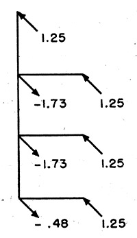
FIG. 21. Current pattern for three border junction.

Networks with Complex Impedances

If both resistances and inductances occur in a network, then the unbalanced junction-currents are complex numbers i₁+ji₂, instead of real numbers i₁. Similarly the absolute potentials are complex numbers. Then a separate current pattern has to be established for a unit change in the real and the imaginary components of junction-voltage respectively. The latter must so change that both the real and imaginary parts of unbalanced currents approach zero.

Another and perhaps a better method is to replace the equivalent circuit by a more complex circuit in which only real numbers occur. Such a step is always possible since a set of differential equations containing complex coefficients may always be replaced by a set containing no j by simply doubling the number of equations and the number of dependent variables, that is, by introducing in-phase and out-of-phase components of variables.


The "Diffusion" Method

While the relaxation and the weighted average methods change potentials at one junction at a time, the method of unbalanced currents and voltages changes the potentials at all junctions simultaneously. The first two methods are found to be effective at the beginning of the reduction, especially in the elimination of "bumps" in otherwise smooth curves; afterwards the latter method appears to be faster. When the unbalanced currents are small compared with the circuit currents but still further reduction is desired, all three methods become very slow. The following method offers a further systematization of the third method.

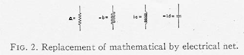
A partial diferential equation, not containing time, usually is considered to represent summation of currents at a junction. An unbalanced current i_u has no counterpart in the equation. Let it be assumed that i_u corresponds to an additional term of the form A∂φ / ∂t in the equation, adding thereby an additional independent variable t to the equation and an additional dimension to the network, such as shown in Fig. 4, for the wave equation.

From physical consideration of diffusion problems, it appears that if the initial conditions are well selected, the rate of diffusion decreases as time increases, and the currents representing A∂φ / ∂t must become in general smaller. At t = oo they all must become zero, allowing the network to represent the original equation without the time-term.



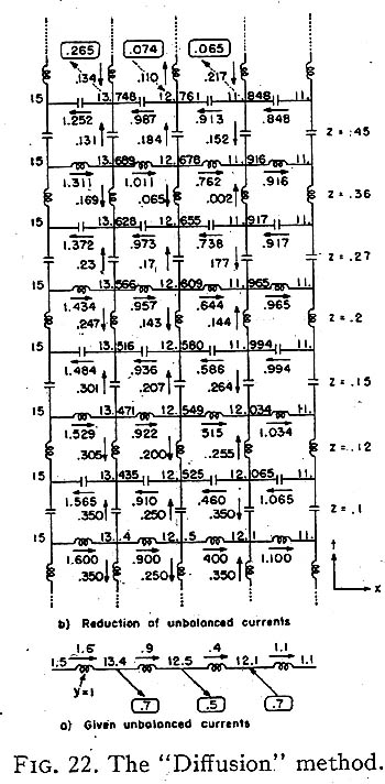
By experience it has been found that at t=0, half of the unbalanced current should flow up, half down (Fig. 22 representing the one-dimensional wave equation). The coefficient A should be so selected that at first the potentials on the second layer should differ by only a small amount (say one percent or less) from the starting potentials. As time goes on, the value of A may be increased to speed up the rate of diffusion. The values of A should be so selected that the bigger currents between the layers should decrease uniformly along smooth-curves instead of oscillate around them. (Some of the smaller currents will increase.) Of course A may be an arbitrary function not only of time, but also of space, allowing thereby speedier diffusion at certain points.

In actual calculations, especially when the layers are two-dimensional, it is sufficient to have the drawing of one layer only and write the subsequent values of potentials in colums, as in the relaxation method.



PART III. CHARACTERISTIC-VALUE PROBLEMS


Oscillatory Circuits

In characteristic-value problems not only the mode of vibration (the junction-potential

distribution) is unknown, but also the frequency ω corresponding to that mode. If, however, a potential distribution is assumed, the corresponding ω may be found by the following property of the networks, a consequence of Rayleigh's Principle.

"When the network potentials correspond to a characteristic function, the algebraic sum of the positive and negative powers in the inductors and capacitors is zero."

That is, the power ΣI²X_L = ΣE²Y_L = ΣEI_L in the inductors is equal to the power ΣI²X_C in the capacitors. Or the power in the variable units, that are functions of ω, is equal to the power in the constant units. This zero power in the network is utilized in finding characteristic values with the aid of a Network Analyzer. The admittances of the coils that are functions of ω are varied with w until a generator, connected in shunt with any of the coils, draws no current from the line. At such values of admittances, the network is self-supporting and the stored electrical energy oscillates between' the capacitors and the inductors.


Calculttion of Characteristic Values

Hence, for an assumed potential distribution e, the corresponding ω is found by the following steps:

1. Calculate the power ΣI²X in all the coils that are not functions of ω (positive power exists in inductors and negative in capacitors)., This power may also be found by calculating the power flowing in the coils that are functions of ω. If the latter are ground coils, then if e is the junction potential and i the current through the ground coils, power = Σei.
2. If the admittance of each of the remaining coils is the same and is equal to ω²C, then the power in these coils is e²y = Σe²ω²C = ω²CΣe². Hence


By Rayleigh's principle it is well known that if the assumed mode of vibration (potentials) is

only a rough approximation, the resultant characteristic value calculated is a better than rough approximation.


By knowing the correct ω for an assumed potential distribution, the correct unbalanced currents i_u and e_u may now be calculated. The latter in turn may be reduced by any of the four methods shown for the solution of boundary- value problems. However, in the present problems a new and more correct ω has to be calculated occasionally as the reduction proceeds.


The Method of Unbalanced Admittances

In the presence of coils that are functions of ω and whose admittances are usually equal, it is not necessary to introduce unbalanced currents. Instead the unbalance is redistributed by attributing different admittances to these variable coils. Hence when the correct ω has been calculated for a given potential distribution, it is assumed that with each variable coil an unbalanced admittance y_u is associated. The purpose of the reduction is then to reduce the values of these unbalanced admittances.

Expressed in another way, the purpose of the reduction is to make the admittances of all variable coils the same. The calculated ω only gives a goal to aim at at the beginning. As the reduction proceeds, the common value of the admittances continuously shifts.

The use of the "unbalanced current patterns" facilitates the calculation of the unbalanced admittances at the neighboring points, when the potential at a point is changed.


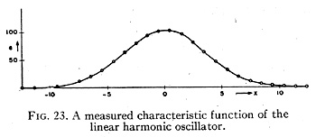
Linear Harmonic Oscillator

It will be assumed that an approximate value of a characteristic function of the linear harmonic oscillator is known, Fig. 23. (Actually it has been measured on a Network Analyzer, (9) with the aid of the network of Fig. 24.)



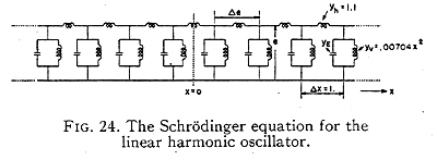
The problem is to calculate the corresponding characteristic value. Theoretically that is known to be y_E=0.0880. zero generator current at y_E=0.0921, a 4 percent discrepancy.

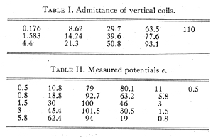
The admittance of the horizontal inductors was Y_h=1.1 and those of the vertical inductors y_v=O.00704x² where x varies from 1/2 to 12 1/2 in steps of 1 as given in Table I for half the coils. The measured potentials from ground to junction are given in Table II.


In the Schrödinger equation the admittance of the capacitors is proportional to ω. The energy in the horizontal coils is Σ1.1∆e² = 2851, in the vertical coils it is fey, Σe²y_v = 2890. Hence



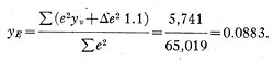
This calculated energy level differs from the theoretical value of 0.0880 by only 3 parts in 10,000. It should also be noted that the true (and lowest) energy level 0.0880 is always smaller than the approximate levels 0.0883 or 0.0921, in accordance with Rayleigh's principle, or its quantum mechanical analogue.



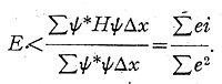
Here ψ is the approximate wave function e. Also H∆xψ is the current i in E∆x the admittance y_E.





BIBLIOGRAPHY

(1) H. W. Emmons, "Numerical methods of solving partial differential equations," Quart. App. Math. (Oct. 1944).

(2) A. Vazsonyi, "Numerical method in the theory of vibrating bodies", J. App. Phys. 15, 598 (1944)

(3) G. Kron, "Equivalent circuits of the elastic field," J. App. Mech. 11, 149-161 (1944).

(4) J.B.Scarborough, "Numerical Mathematical Analysis (Oxford University Press, 1930).

R. E. Doherty and E. Keller, Mathematics of Modern Engineering I (John Wiley & Sons, Inc, New York, 1936), p. 167.

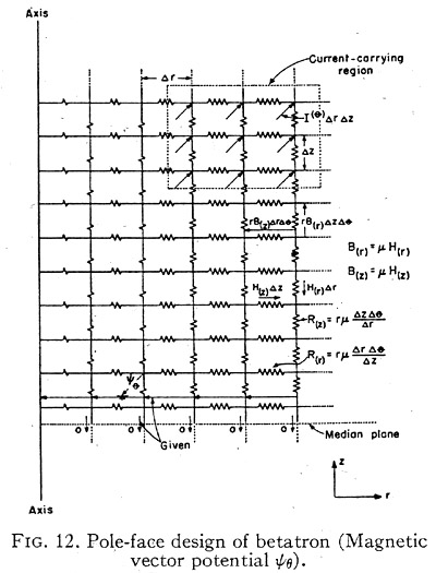
(6) J. H. Bartlett, "The shaping of pole faces of the betatron," Phys. Rev. 63, 185 (1943).

(7) G. Kron, "Equivalent circuits of compressible and incompressible flow fields," scheduled to appear in J. Aer. Sci.

(8) G. K. Carter; "Numerical and network ~.nalyzer solutions of the equivalent circuits for the elastic field;" J. App. Mech. 11,162—167 (1944).

(9) G. K. Carter. and G. Kron, "A.c. network analizer study of the Schrödinger equation," Phys. Rev. 67, 44 (1945).

(10) G. Kron, "Electric circuit models of the Schrödinger equation," Phys. Rev. 67, 39 (1945).

(11) G. Kron, "Equivalent circuit of the field equations of Maxwell," Proc. I. R. E., pp. 289 - 299 (May, 1944).

(12) R. V. Southwell, Relaxation Methods in Engineering Science (Oxford University Press, 1940).

(13) A. F. Prebus, I. Zlotowsky and G. Kron, "The application of network analysis to some electron optical problems," scheduled, to appear in Phys. Rev.